Added thermal tests with ADC clock modifications....

Added thermal tests with ADC clock modifications. Signed-off-by: Alexis Jeandet <alexis.jeandet@member.fsf.org>

jeandet - - Load All Authors

File last commit:

r11:ea8683773e38


                r11:ea8683773e38

Download file

             LFR_CLK_SIMULATION.ipynb
        
                    778 lines
            
             | 2.6 MiB
            
                | text/plain
            
             |
                TextLexer

/ LFR_CLK_SIMULATION / LFR_CLK_SIMULATION.ipynb

History | Annotation | Raw |Copy content |Copy permalink

LFR ADC CLK simulations¶

Context¶

EQM clk model¶

To get a better understanding of LFR's ADC clk issue, a modelisation and a simulation of the clock line seems important. Fisrt let's have a look to its topology:

LFR PCB

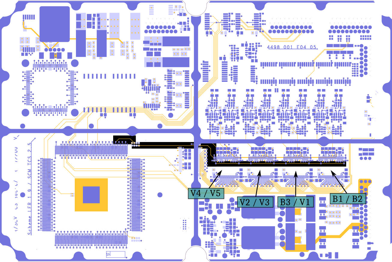
To extract the equivalent model of thec CLK line, we have to modelize PCB track and ADC input pins. A PCB trac can be decomposed in a R L C circuit. At this time we will mainly focuss on L since it's resistance is small compared to discrete component in the circuit, while C might be hard to extrac since it depends on PCB materail and has a complex shape.

From the datasheet the RHF1401is said to have a 7pF input capacitance.

ADC Clock equivalent diagram

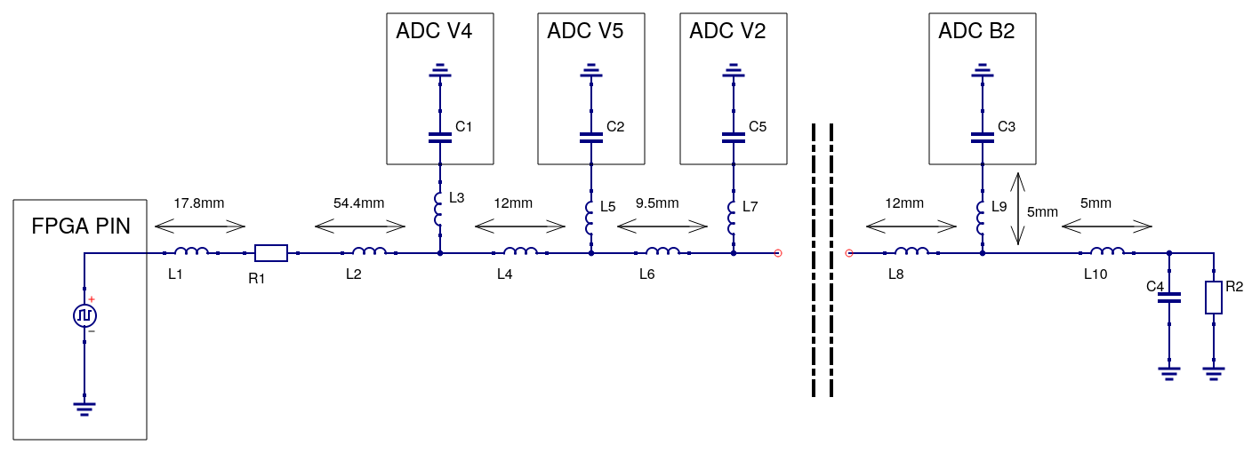
R1 is equivalent to R82,R83,R84 on EQM which are 3 470Ohm in parallel, R2 is equivalent to R85 (470Ohm) and C4 is 220pF (manually added on EQM).

Track inductance evaluation¶

Using the following formula we can evaluate PCB inductance:

\begin{equation*} Inductance(\mu H) = 2 \times 10^{-3} \times L \times [ ln( \frac{ 2 \times L}{W + T} ) + 0.5 + 0.2235 \times (\frac{W + T}{L}) ] \end{equation*}

PCB track

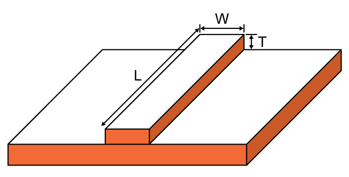
On LFR EQM W = 200 µm and T = 35µm for inner layers and 18µm for outer layers. This gives:

L1 = 19.6nH ((17.8mm/35µm/200µm))
L2 = 72nH (54.4mm/35µm/200µm)
L3/L5/L7/L9 = 4.35nH (5mm/18µm/200µm)
L4/L8 = 12nH (12mm/35µm/200µm)
L6 = 9.3nH (9.5mm/35µm/200µm)
L10 = 2.8 (5mm/500µm/500µm)

Simplified model¶

EQM Simulation results¶

Reference simulation¶

The circuit is simulated with QUCS in time domain from 1µs to 2µs with a 10ps step. The FPGA output signal is a 1MHz/3.3V square signal with 1ns rise and fall time.

In [1]:

%matplotlib inline
import matplotlib.pyplot as plt
import matplotlib
import sys
import numpy as np
import pandas as pds
from glob import glob
from IPython.display import display
from dateutil import parser
from IPython.display import HTML,Markdown,Math
from IPython.display import display

def plot_temperatures(file):
    temperature=pds.read_csv(file, sep='\t', index_col=0,parse_dates=True)
    temperature.plot(figsize=(24,10))
    plt.show()


font = {'family' : 'DejaVu Sans',
        'weight' : 'bold',
        'size'   : 18}

matplotlib.rc('font', **font)

HTML('''<script>
code_show=true; 
function code_toggle() {
 if (code_show){
 $('div.input').hide();
 } else {
 $('div.input').show();
 }
 code_show = !code_show
} 
$( document ).ready(code_toggle);
</script>
 <a href="javascript:code_toggle()"><font size="6">Show/Hide code</font></a>.''')

Out[1]:

Show/Hide code.

In [2]:

fig,ax=plt.subplots(4,2, figsize=(40,30))
pds.read_csv("./Simulations/EQM_MODEL/V5.csv", sep=';', index_col=0)["r V5.Vt"][1.4e-06:1.6e-06].plot(ax=ax[0][0], label="V5",legend=True)
pds.read_csv("./Simulations/EQM_MODEL/V4.csv", sep=';', index_col=0)["r V4.Vt"][1.4e-06:1.6e-06].plot(ax=ax[0][1], label="V4",legend=True)
pds.read_csv("./Simulations/EQM_MODEL/V3.csv", sep=';', index_col=0)["r V3.Vt"][1.4e-06:1.6e-06].plot(ax=ax[1][0], label="V3",legend=True)
pds.read_csv("./Simulations/EQM_MODEL/V2.csv", sep=';', index_col=0)["r V2.Vt"][1.4e-06:1.6e-06].plot(ax=ax[1][1], label="V2",legend=True)
pds.read_csv("./Simulations/EQM_MODEL/V1.csv", sep=';', index_col=0)["r V1.Vt"][1.4e-06:1.6e-06].plot(ax=ax[2][0], label="V1",legend=True)
pds.read_csv("./Simulations/EQM_MODEL/B3.csv", sep=';', index_col=0)["r B3.Vt"][1.4e-06:1.6e-06].plot(ax=ax[2][1], label="B3",legend=True)
pds.read_csv("./Simulations/EQM_MODEL/B2.csv", sep=';', index_col=0)["r B2.Vt"][1.4e-06:1.6e-06].plot(ax=ax[3][0], label="B2",legend=True)
pds.read_csv("./Simulations/EQM_MODEL/B1.csv", sep=';', index_col=0)["r B1.Vt"][1.4e-06:1.6e-06].plot(ax=ax[3][1], label="B1",legend=True)
plt.tight_layout()

We can see on this plots that B2 ADC see a clean clock signal while V5/V4 has a really disturbed one. This is coherent with what we observe on PFM board and EQM, most poluted channels are V5 and V4. One other observation is that the square slope is quite slow due to C4 and all ADC inputs, we can simulate hat append if we remove C4.

Simulation without C4¶

This simulation is done with exactly the same parameters than the reference one.

In [3]:

fig,ax=plt.subplots(4,2, figsize=(40,30))
pds.read_csv("./Simulations/EQM_MODEL_WITHOUT_C4/V5.csv", sep=';', index_col=0)["r V5.Vt"][1.4e-06:1.6e-06].plot(ax=ax[0][0], label="V5",legend=True)
pds.read_csv("./Simulations/EQM_MODEL_WITHOUT_C4/V4.csv", sep=';', index_col=0)["r V4.Vt"][1.4e-06:1.6e-06].plot(ax=ax[0][1], label="V4",legend=True)
pds.read_csv("./Simulations/EQM_MODEL_WITHOUT_C4/V3.csv", sep=';', index_col=0)["r V3.Vt"][1.4e-06:1.6e-06].plot(ax=ax[1][0], label="V3",legend=True)
pds.read_csv("./Simulations/EQM_MODEL_WITHOUT_C4/V2.csv", sep=';', index_col=0)["r V2.Vt"][1.4e-06:1.6e-06].plot(ax=ax[1][1], label="V2",legend=True)
pds.read_csv("./Simulations/EQM_MODEL_WITHOUT_C4/V1.csv", sep=';', index_col=0)["r V1.Vt"][1.4e-06:1.6e-06].plot(ax=ax[2][0], label="V1",legend=True)
pds.read_csv("./Simulations/EQM_MODEL_WITHOUT_C4/B3.csv", sep=';', index_col=0)["r B3.Vt"][1.4e-06:1.6e-06].plot(ax=ax[2][1], label="B3",legend=True)
pds.read_csv("./Simulations/EQM_MODEL_WITHOUT_C4/B2.csv", sep=';', index_col=0)["r B2.Vt"][1.4e-06:1.6e-06].plot(ax=ax[3][0], label="B2",legend=True)
pds.read_csv("./Simulations/EQM_MODEL_WITHOUT_C4/B1.csv", sep=';', index_col=0)["r B1.Vt"][1.4e-06:1.6e-06].plot(ax=ax[3][1], label="B1",legend=True)
plt.tight_layout()

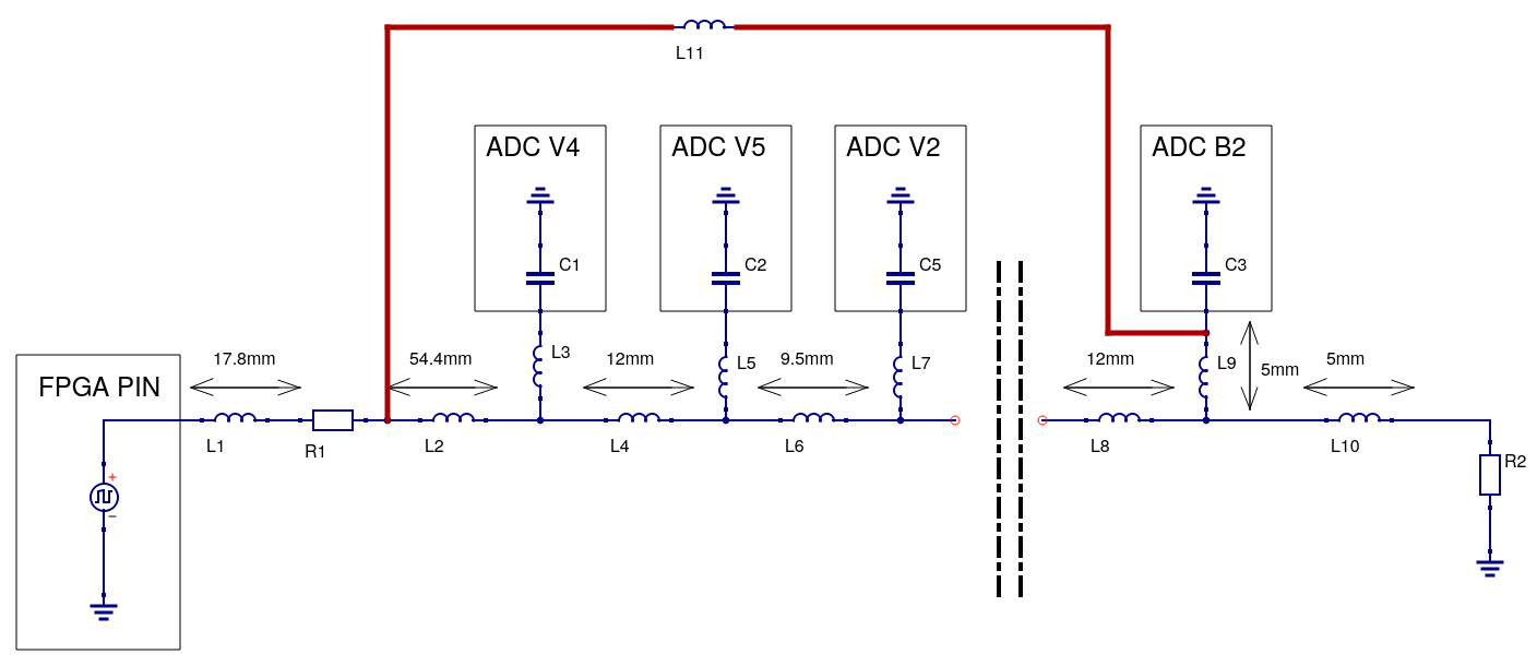
Removing C4 does really improves the clock slope and the overal signal but we still have oscillations around VDD/2 witch may lead to the actual bug. After many tests on a simplified model we came to the conclusion that adding an inductance between R1 and C3 has a really good effect on clk signal. This could be implemented by soldering a wire between R1 and B2 ADC clk pin, length and section of the wire has to be choosen to be as close as possible to L2(72nH).

Solution simulation¶

New equivalent model¶

ADC Clock equivalent diagram

Simulation results¶

The distance between R1 and the the B2 ADC is about 15cm, a 800µm diameter wire would give us 180nH which is too much. In order to show the efficiency of this solutiuon, we will use a 100nH wire and we will see later how get this value.

In [4]:

fig,ax=plt.subplots(4,2, figsize=(40,30))
pds.read_csv("./Simulations/EQM_MODEL_WITHOUT_C4_Wire/V5.csv", sep=';', index_col=0)["r V5.Vt"][1.4e-06:1.6e-06].plot(ax=ax[0][0], label="V5",legend=True)
pds.read_csv("./Simulations/EQM_MODEL_WITHOUT_C4_Wire/V4.csv", sep=';', index_col=0)["r V4.Vt"][1.4e-06:1.6e-06].plot(ax=ax[0][1], label="V4",legend=True)
pds.read_csv("./Simulations/EQM_MODEL_WITHOUT_C4_Wire/V3.csv", sep=';', index_col=0)["r V3.Vt"][1.4e-06:1.6e-06].plot(ax=ax[1][0], label="V3",legend=True)
pds.read_csv("./Simulations/EQM_MODEL_WITHOUT_C4_Wire/V2.csv", sep=';', index_col=0)["r V2.Vt"][1.4e-06:1.6e-06].plot(ax=ax[1][1], label="V2",legend=True)
pds.read_csv("./Simulations/EQM_MODEL_WITHOUT_C4_Wire/V1.csv", sep=';', index_col=0)["r V1.Vt"][1.4e-06:1.6e-06].plot(ax=ax[2][0], label="V1",legend=True)
pds.read_csv("./Simulations/EQM_MODEL_WITHOUT_C4_Wire/B3.csv", sep=';', index_col=0)["r B3.Vt"][1.4e-06:1.6e-06].plot(ax=ax[2][1], label="B3",legend=True)
pds.read_csv("./Simulations/EQM_MODEL_WITHOUT_C4_Wire/B2.csv", sep=';', index_col=0)["r B2.Vt"][1.4e-06:1.6e-06].plot(ax=ax[3][0], label="B2",legend=True)
pds.read_csv("./Simulations/EQM_MODEL_WITHOUT_C4_Wire/B1.csv", sep=';', index_col=0)["r B1.Vt"][1.4e-06:1.6e-06].plot(ax=ax[3][1], label="B1",legend=True)
plt.tight_layout()

In [5]:

pds.read_csv("./Simulations/EQM_MODEL_WITHOUT_C4_Wire/B1.csv", sep=';')[40000:40004].time

Out[5]:

40000    0.000001
40001    0.000001
40002    0.000001
40003    0.000001
Name: time, dtype: float64

Even though the result aren't perfect, we can see an improvement on the clock signal.

Conclusion¶

Removing the 220pF capacitor and adding a wire between R82/3/4 and B2 ADC(U21) should solve the issue. This modification must be tested on the EQM to show the validity of this solution and the simulations.

Measurements on EQM¶

With and without strap measurements and comparaison¶

In [6]:

fig,ax=plt.subplots(4,2, figsize=(40,30), sharex=True, sharey=True)
pds.read_csv("./Measurements/C1EQM_CLK_V5_NO_STRAP_NO_CAP00000.txt", sep='\t', skiprows=4, index_col=0)[-6.0e-7:-3.5e-7].plot(ax=ax[0][0], label="V5",legend=True)
pds.read_csv("./Measurements/C1EQM_CLK_V4_NO_STRAP_NO_CAP00000.txt", sep='\t', skiprows=4, index_col=0)[-6.0e-7:-3.5e-7].plot(ax=ax[0][1], label="V4",legend=True)
pds.read_csv("./Measurements/C1EQM_CLK_V3_NO_STRAP_NO_CAP00000.txt", sep='\t', skiprows=4, index_col=0)[-6.0e-7:-3.5e-7].plot(ax=ax[1][0], label="V3",legend=True)
pds.read_csv("./Measurements/C1EQM_CLK_V2_NO_STRAP_NO_CAP00000.txt", sep='\t', skiprows=4, index_col=0)[-6.0e-7:-3.5e-7].plot(ax=ax[1][1], label="V2",legend=True)
pds.read_csv("./Measurements/C1EQM_CLK_V1_NO_STRAP_NO_CAP00000.txt", sep='\t', skiprows=4, index_col=0)[-6.0e-7:-3.5e-7].plot(ax=ax[2][0], label="V1",legend=True)
pds.read_csv("./Measurements/C1EQM_CLK_B3_NO_STRAP_NO_CAP00000.txt", sep='\t', skiprows=4, index_col=0)[-6.0e-7:-3.5e-7].plot(ax=ax[2][1], label="B3",legend=True)
pds.read_csv("./Measurements/C1EQM_CLK_B2_NO_STRAP_NO_CAP00000.txt", sep='\t', skiprows=4, index_col=0)[-6.0e-7:-3.5e-7].plot(ax=ax[3][0], label="B2",legend=True)
pds.read_csv("./Measurements/C1EQM_CLK_B1_NO_STRAP_NO_CAP00000.txt", sep='\t', skiprows=4, index_col=0)[-6.0e-7:-3.5e-7].plot(ax=ax[3][1], label="B1",legend=True)

pds.read_csv("./Measurements/C1EQM_CLK_V5_WITH_STRAP_NO_CAP00000.txt", sep='\t', skiprows=4, index_col=0)[-6.0e-7:-3.5e-7].plot(ax=ax[0][0], label="V5",legend=True)
pds.read_csv("./Measurements/C1EQM_CLK_V4_WITH_STRAP_NO_CAP00000.txt", sep='\t', skiprows=4, index_col=0)[-6.0e-7:-3.5e-7].plot(ax=ax[0][1], label="V4",legend=True)
pds.read_csv("./Measurements/C1EQM_CLK_V3_WITH_STRAP_NO_CAP00000.txt", sep='\t', skiprows=4, index_col=0)[-6.0e-7:-3.5e-7].plot(ax=ax[1][0], label="V3",legend=True)
pds.read_csv("./Measurements/C1EQM_CLK_V2_WITH_STRAP_NO_CAP00000.txt", sep='\t', skiprows=4, index_col=0)[-6.0e-7:-3.5e-7].plot(ax=ax[1][1], label="V2",legend=True)
pds.read_csv("./Measurements/C1EQM_CLK_V1_WITH_STRAP_NO_CAP00000.txt", sep='\t', skiprows=4, index_col=0)[-6.0e-7:-3.5e-7].plot(ax=ax[2][0], label="V1",legend=True)
pds.read_csv("./Measurements/C1EQM_CLK_B3_WITH_STRAP_NO_CAP00000.txt", sep='\t', skiprows=4, index_col=0)[-6.0e-7:-3.5e-7].plot(ax=ax[2][1], label="B3",legend=True)
pds.read_csv("./Measurements/C1EQM_CLK_B2_WITH_STRAP_NO_CAP00000.txt", sep='\t', skiprows=4, index_col=0)[-6.0e-7:-3.5e-7].plot(ax=ax[3][0], label="B2",legend=True)
pds.read_csv("./Measurements/C1EQM_CLK_B1_WITH_STRAP_NO_CAP00000.txt", sep='\t', skiprows=4, index_col=0)[-6.0e-7:-3.5e-7].plot(ax=ax[3][1], label="B1",legend=True)
fig.subplots_adjust(hspace=0, wspace=0)

Simulations and measurement comparaisons¶

In [7]:

fig,axes=plt.subplots(4,2, figsize=(40,30), sharex=True, sharey=True)
for ch,ax in [ ("V5", axes[0][0]), ("V4", axes[0][1]), ("V3", axes[1][0]), ("V2", axes[1][1]), ("V1", axes[2][0]), ("B3", axes[2][1]), ("B2", axes[3][0]), ("B1", axes[3][1])]:
    measurement_no_strap = pds.read_csv("./Measurements/C1EQM_CLK_{ch}_NO_STRAP_NO_CAP00000.txt".format(ch=ch), sep='\t', skiprows=4, index_col=0)[-6.0e-7:-3.5e-7]["Ampl"]
    measurement_no_strap.index += 1.990e-06
    measurement_no_strap.plot(ax=ax, label="{ch}_Measure_no_wire".format(ch=ch),legend=True, linewidth=3)
    
    measurement_with_strap = pds.read_csv("./Measurements/C1EQM_CLK_{ch}_WITH_STRAP_NO_CAP00000.txt".format(ch=ch), sep='\t', skiprows=4, index_col=0)[-6.0e-7:-3.5e-7]["Ampl"]
    measurement_with_strap.index += 1.999e-06
    measurement_with_strap.plot(ax=ax, label="{ch}_Measure_with_wire".format(ch=ch),legend=True, linewidth=3)
    
    measurement_with_270_Ohms_strap = pds.read_csv("./Measurements/C1EQM_CLK_{ch}_WITH_STRAP_270_OHMS_NO_CAP00000.txt".format(ch=ch), sep='\t', skiprows=4, index_col=0)[-6.0e-7:-3.5e-7]["Ampl"]
    measurement_with_270_Ohms_strap.index += 2.008e-06
    measurement_with_270_Ohms_strap.plot(ax=ax, label="{ch}_Measure_with_wire_270_Ohms".format(ch=ch),legend=True, linewidth=3)

    simu_with_strap = pds.read_csv("./Simulations/EQM_MODEL_WITHOUT_C4_Wire/{ch}.csv".format(ch=ch), sep=';', index_col=0)
    simu_with_strap.index -= 2.e-8
    simu_with_strap["r {ch}.Vt".format(ch=ch)][1.4e-06:1.6e-06].plot(ax=ax, label="{ch}_Simu_With_Wire".format(ch=ch),legend=True, linewidth=3)

    simu_no_strap = pds.read_csv("./Simulations/EQM_MODEL_WITHOUT_C4/{ch}.csv".format(ch=ch), sep=';', index_col=0)
    simu_no_strap.index -= 1e-8
    simu_no_strap["r {ch}.Vt".format(ch=ch)][1.4e-06:1.6e-06].plot(ax=ax, label="{ch}_Simu_No_Wire".format(ch=ch),legend=True, linewidth=3)
fig.subplots_adjust(hspace=0, wspace=0)

Thermal tests¶

Default conf (No Wire, C4 present)¶

In [22]:

plot_temperatures("/home/jeandet/ownCloud/TESTS_LFR_EQM2_LABO_BUG_BIAS4/temperature_21_09_2017.log")

In [19]:

!mkdir -p "/home/jeandet/ownCloud/TESTS_LFR_EQM2_LABO_BUG_BIAS4/analysis/pictures/2017_09_21"
%run /home/jeandet/ownCloud/TESTS_LFR_EQM2_LABO_BUG_BIAS4/analysis/LFR_Thermal_Cycling_ADC_Bug.py "/home/jeandet/Documents/DATA/LFR_Packets/" "2017_09_21_14_38_21" "2017_09_21_14_38_20" "/home/jeandet/ownCloud/TESTS_LFR_EQM2_LABO_BUG_BIAS4/temperature_21_09_2017.log" "/home/jeandet/ownCloud/TESTS_LFR_EQM2_LABO_BUG_BIAS4/analysis/pictures/2017_09_21"

In [20]:

%%capture
!cd /home/jeandet/ownCloud/TESTS_LFR_EQM2_LABO_BUG_BIAS4/analysis/pictures/2017_09_21 && ffmpeg -y -framerate 15 -i plot_%d.png video.mp4 && ffmpeg -y -i video.mp4 -c:v libvpx-vp9 -b:v 2M -threads 8 video.webm

In [36]:

%%HTML
<video width="90%" style="display:block; margin: 0 auto;" controls src="https://hephaistos.lpp.polytechnique.fr/data/LFR/LFR_ADC_BUG_INVESTIGATION/pictures/2017_09_21/video.webm" type="video/webm">

Conf 1, wire soldered and C4 removed.¶

In [26]:

plot_temperatures("/home/jeandet/ownCloud/TESTS_LFR_EQM2_LABO_BUG_BIAS4/temperature_25_09_2017.log")

In [27]:

!mkdir -p "/home/jeandet/ownCloud/TESTS_LFR_EQM2_LABO_BUG_BIAS4/analysis/pictures/2017_09_25"
%run /home/jeandet/ownCloud/TESTS_LFR_EQM2_LABO_BUG_BIAS4/analysis/LFR_Thermal_Cycling_ADC_Bug.py "/home/jeandet/Documents/DATA/LFR_Packets/" "2017_09_25_14_47_03" "2017_09_25_14_47_02" "/home/jeandet/ownCloud/TESTS_LFR_EQM2_LABO_BUG_BIAS4/temperature_25_09_2017.log" "/home/jeandet/ownCloud/TESTS_LFR_EQM2_LABO_BUG_BIAS4/analysis/pictures/2017_09_25"

<matplotlib.figure.Figure at 0x7f04a4f4b5f8>

In [28]:

%%capture
!cd /home/jeandet/ownCloud/TESTS_LFR_EQM2_LABO_BUG_BIAS4/analysis/pictures/2017_09_25 && ffmpeg -y -framerate 15 -i plot_%d.png video.mp4 && ffmpeg -y -i video.mp4 -c:v libvpx-vp9 -b:v 2M -threads 8 video.webm

In [35]:

%%HTML
<video width="90%" style="display:block; margin: 0 auto;" controls src="https://hephaistos.lpp.polytechnique.fr/data/LFR/LFR_ADC_BUG_INVESTIGATION/pictures/2017_09_25/video.webm" type="video/webm">

Conf 2, same as conf 1 but R1=90 $\Omega$ and R2=270 $\Omega$¶

In [30]:

plot_temperatures("/home/jeandet/ownCloud/TESTS_LFR_EQM2_LABO_BUG_BIAS4/temperature_29_09_2017.log")

In [31]:

!mkdir -p "/home/jeandet/ownCloud/TESTS_LFR_EQM2_LABO_BUG_BIAS4/analysis/pictures/2017_09_29"
%run /home/jeandet/ownCloud/TESTS_LFR_EQM2_LABO_BUG_BIAS4/analysis/LFR_Thermal_Cycling_ADC_Bug.py "/home/jeandet/Documents/DATA/LFR_Packets/" "2017_09_29_15_45_01" "2017_09_29_15_45_01" "/home/jeandet/ownCloud/TESTS_LFR_EQM2_LABO_BUG_BIAS4/temperature_29_09_2017.log" "/home/jeandet/ownCloud/TESTS_LFR_EQM2_LABO_BUG_BIAS4/analysis/pictures/2017_09_29"

<matplotlib.figure.Figure at 0x7f04a4afa080>

In [32]:

%%capture
!cd /home/jeandet/ownCloud/TESTS_LFR_EQM2_LABO_BUG_BIAS4/analysis/pictures/2017_09_29 && ffmpeg -y -framerate 15 -i plot_%d.png video.mp4 && ffmpeg -y -i video.mp4 -c:v libvpx-vp9 -b:v 2M -threads 8 video.webm

In [34]:

%%HTML
<video width="90%" style="display:block; margin: 0 auto;" controls src="https://hephaistos.lpp.polytechnique.fr/data/LFR/LFR_ADC_BUG_INVESTIGATION/pictures/2017_09_29/video.webm" type="video/webm">

	Site-wide shortcuts
/	Use quick search box
g h	Goto home page
g g	Goto my private gists page
g G	Goto my public gists page
g 0-9	Goto bookmarked items from 0-9
n r	New repository page
n g	New gist page

	Repositories
g s	Goto summary page
g c	Goto changelog page
g f	Goto files page
g F	Goto files page with file search activated
g p	Goto pull requests page
g o	Goto repository settings
g O	Goto repository access permissions settings
t s	Toggle sidebar on some pages